神经网络案例展示
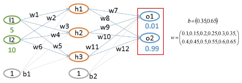
1 题目:
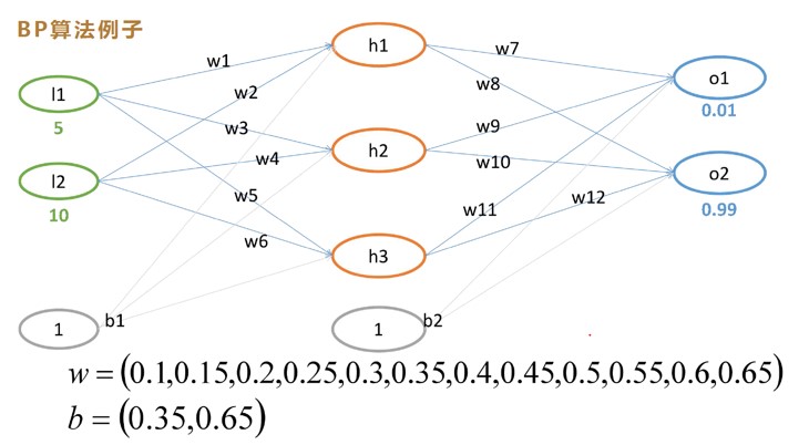
其中:
l1 和 l2 为 inputs
wi 和 bi 为 weights
o1 和 o2 为 outputs
o1 的label 为 0.01,o2 的 label 为 0.99
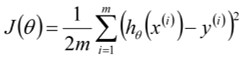
损失函数我们使用MSELoss:
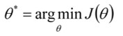
我们的优化目标为:
2 前向传播过程(feedforward)
2.1 第一层求解
- 线性变换
- 非线性变换(激活函数)
- 同理可得:
2.2 第二层计算
- 线性变换
- 分析性变换(激活函数)
- 同理可得:
- 总误差为:
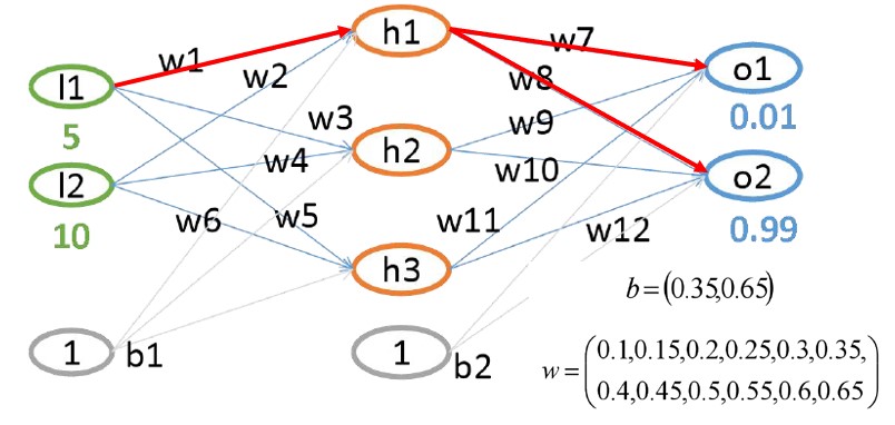
3 反向传播过程(back propagation)
3.1 末层权重梯度计算
- 以 梯度计算为例:
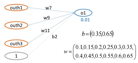
3.1.1 计算流程概述
- 前向过程为:
--> 线性连接 --> --> 激活 --> --> MSELoss -->
- 反向过程为:
3.1.2 具体计算过程
- 误差对 的梯度计算
- 激活函数导数计算
- 线性项导数计算
- 链式求导:
- 同理可求得 w_{8}、 w_{9}、 w_{10}、 w_{11}、 w_{12} 的梯度
3.2 前一层权重梯度计算(以 梯度计算为例)
- 核心公式
- 其中:
- 带入数据:
- 同理可求的 , 于是可得到:
- 同理可求得 w_{2}、 w_{3}、 w_{4}、 w_{5}、 w_{6} 的梯度。
4 权重更新
- 更新 :
- 同理可得:
5 迭代训练
- 第10次迭代结果:
- 第100次迭代结果:
- 第1000次迭代结果:
- 1000次时对应的权重为:
思考:不同的训练参数,最后的权重 和 O 趋于一致吗 ???
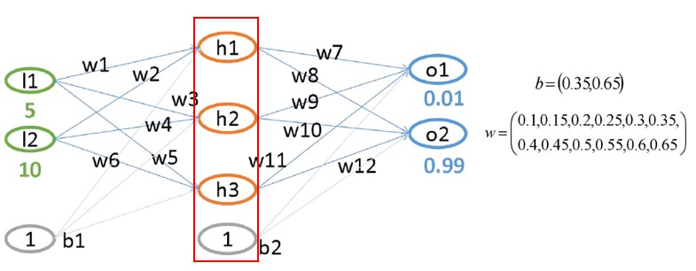
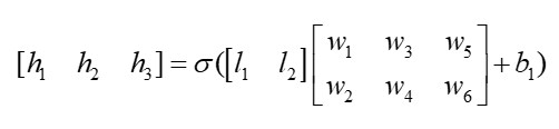
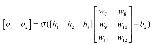
6 将前馈网络写成矩阵形式
第一层:
第二层:
7 代码展示
python
'''
如果 X W 两个矩阵:
W[n,k] @ X[k,m] = Y[n,m] #
则: dW = dY @ XT; dX = WT @ dY #  矩阵反向传播公式
output = a + b
'''
import numpy as np

def bp_demo():
    def sigmoid(input):
        return 1 / (1 + np.e**(-input))

    def sigmoid_backward(out):
        return out*(1- out)

    w1 = np.array([[0.1, 0.15], [0.2, 0.25], [0.3, 0.35]])
    w2 = np.array([[0.4, 0.45, 0.5], [0.55, 0.6, 0.65]])
    b1 = 0.35
    b2 = 0.65
    input = np.array([5, 10]).reshape(2, 1)
    label = np.array([0.01, 0.99]).reshape(2, 1)

    for i in range(100):
        net_h = w1 @ input + b1
        out_h = sigmoid(net_h)

        net_o = w2 @ out_h + b2
        out_o = sigmoid(net_o)

        loss = np.sum((out_o - label)**2)
        print(loss)

        dw2 = (out_o - label) * sigmoid_backward(out_o) @ out_h.T

        # (out_o - label) * sigmoid_backward(out_o) --> dloss/net_o
        dout_h = w2.T @ ((out_o - label) * sigmoid_backward(out_o))

        dw1 = dout_h * sigmoid_backward(out_h) @ input.T

        w1 = w1 - 0.5 * dw1
        w2 = w2 - 0.5 * dw2
        print(f"loss[{i}]: {loss}")

    print(w1)


def matmul_grad():
    W = np.array([[4, 5], [7, 2]])
    X = np.array([2, 6.0]).reshape(2, 1)
    label = np.array([14, 11]).reshape(2, 1)

    for i in range(100):
        Y = W @ X # 线性相乘
        Loss = 0.5 * np.sum((Y-label)**2) # 损失值 --> 标量
        # dY = Y - label # 向量
        dW = (Y-label) @ X.T # 矩阵求导公式
        W = W - 0.01*dW # 更新weight
        print(f"============= loss[{i}]: ", Loss)

    print(W)

def loss_grad(o1, o2, label):
    # loss = (o1 - 14)**2 + (o2 -11)**2 # 距离越远,值越大
    # Loss = np.sum((O - Lable)**2)
    grad = [2 * (o1 - label[0]), 2 * (o2 - label[1])]
    return np.array(grad)

def matrix_grad_demo():
    """
      4x + 5y = O1
      7x + 2y = O1

      [[4, 5], [7, 2]] * [x, y]T = [01, 02] --> A*x = O
      label = [14, 11] # 代表我们期望的那个值
      loss = (o1 - 14)**2 + (o2 -11)**2 # 距离越远,值越大
    """
    A = np.array([[4.0, 5], [7.0, 2]])
    X = np.array([2, 6.0]) # 随便给的初始值

    Lable = np.array([14, 11])
    lr = 0.001

    for i in range(1000):
        O = A @ X   # 前向
        grad = A.T @ loss_grad(O[0], O[1], Lable)
        X[0] = X[0] - lr*grad[0]
        X[1] = X[1] - lr*grad[1]
        print("x[0]: {}, x[1]: {}".format(X[0], X[1]))
        Loss = np.sum((O - Lable)**2)
        print("Loss: ", Loss)

if __name__ == "__main__":
    # matrix_grad_demo()
    # matmul_grad()
    bp_demo()
    print("run grad_descend.py successfully !!!")